Quantum Signal Processing and Grover's Search
On May 6th, 2021, Chuang et al. posted the paper A Grand Unification of Quantum Algorithms which claims that arguably the three most important algorithms in quantum computing: search, factoring and simulation, all have a common underlying structure: the quantum singular value transform. In this pedagogical paper, based heavily on work by Gilyen et al., they explain this structure, starting out with a primitive called quantum signal processing, which leads to the quantum eigenvalue transformation, and finally, the coveted quantum singular value transformation.
This article covers my take on the first part of this review: quantum signal processing, and how Grover’s search emerges from it.
We’ll organise this into three sections:
- Quantum signal processing (QSP): This is a transformation that is defined for single qubit operations.
- Generalising QSP: How the above transformation is defined for any operation (even those that act on more than one qubit), as long as you care about their action on a small space. Chuang et al. call this portion amplitude amplification.
- Grover’s search from the generalised QSP: How the Grover’s search is basically the QSP, with some constraints on it.
Quantum Signal Processing (QSP)
As the name suggests, quantum signal processing is a transformation that takes a signal and processes it and either the signal or the processing or both are quantum things.
Alright, let’s get precise. By signal, we mean a rotation by an angle \(\theta\) about the \(X\) axis of the Bloch sphere. Just so we have the same picture, here is the (slightly wobbly) Bloch sphere that I’m going to be referring to.
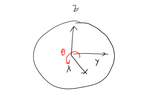
The unitary representing this rotation is given by \(e^{-i\frac{\theta}{2}\sigma_x}\) where \(\sigma_x\) is the Pauli matrix \(\begin{bmatrix} 0 & 1 \\ 1 & 0 \\ \end{bmatrix}\). It turns out to be convenient to consider this \(\theta\) to be \(-2 \operatorname{cos}^{-1} a\), and write this rotation matrix in terms of \(a\):
\[W(a) = \begin{bmatrix} a & i\sqrt{1 - a^2} \\ i\sqrt{1 - a^2} & a \\ \end{bmatrix}\]The processing of the signal refers to manipulation of the signal by multiplying it with other matrices. The precise way in which this is done is we interleave the signal with \(Z\)-rotation matrices. That is, matrices of the form \(e^{-i \frac{\phi}{2} \sigma_z}\), where \(\sigma_z\) is \(\begin{bmatrix} 1 & 0 \\ 0 & -1 \end{bmatrix}\). We’ll denote these rotations by \(R_z(\phi)\).
Thus, the circuit obtained upon processing the signal looks like
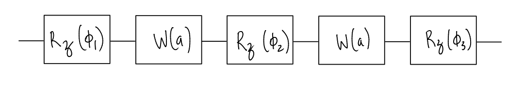
Let’s call a circuit of the above form \(Q\), and let the number of applications of \(W(a)\) in \(Q\) be \(d\). Then, the quantum signal processing theorem crudely states1:
- For any \(Q\), we have \(\langle 0 \vert Q \vert 0\rangle\) is a polynomial in \(a\) with degree \(\leq d\).
- It is possible to obtain, for any polynomial \(P(a)\) with degree \(\leq d\), a set of \(d+1\) phases \(\{\phi_i\}_i\) such that a \(Q\) prepared using this phases as the \(Z\)-rotations will have \(\langle 0 \vert Q \vert 0 \rangle = P(a)\).
Moreover, for any polynomial \(P\), there exist efficient classical algorithms to obtain these phases. In fact, Chuang’s paper comes with a package that computes these phases for you!
Now, why might it be useful to do this? Let us think about this for a minute even before we look at some applications. Assume that we are given some input signal, represented by the parameter \(a\), which we know nothing about. Then, we have the ability to manipulate that signal to get a circuit \(Q\) to obtain some information about \(a\), by choosing \(\langle 0 \vert Q \vert 0\rangle\) to be an appropriate polynomial in \(a\). Indeed, in the paper, an example of a polynomial that has a high value for some inputs \(a\), but a low value for others is provided. Thus, one could guess information about \(a\), by manipulating the input signal and estimating the entry value of \(\langle 0 \vert Q \vert 0 \rangle\) using measurement.
However, the really cool application is that Grover’s search emerges beautifully from this idea of signal manipulation. To see that, we have to first generalise the QSP to higher dimensions.
Generalising the QSP
Let’s leave our happy \(2\)-dimensional space, and consider some arbitrary finite dimensional Hilbert space \(\mathcal{H}\). Assume someone provides you with the following three operators:
- Some unitary matrix \(U\) which acts on \(\mathcal{H}\).
- Operators of the form \(e^{i \phi \vert A_0 \rangle \langle A_0 \vert}\), for any \(\phi\)’s that you please, but a fixed \(\vert A_0 \rangle\).
- Analogously, operators of the form \(e^{i \phi \vert B_0 \rangle \langle B_0 \vert}\), for any \(\phi\)’s that you please, but a fixed \(\vert B_0 \rangle\).
Aaaand, you’ve been promised that \(a \equiv \langle A_0 \vert U \vert B_0 \rangle \neq 0\).2
In any case, by giving you these three powers, they’ve given you: the ability to create a circuit \(Q\) such that \(\langle A_0 \vert Q \vert B_0 \rangle = P(a)\), for any polynomial \(P\) that you want, as long as it satisfies the same constraints as that of the signal processing theorem. But how does this work?
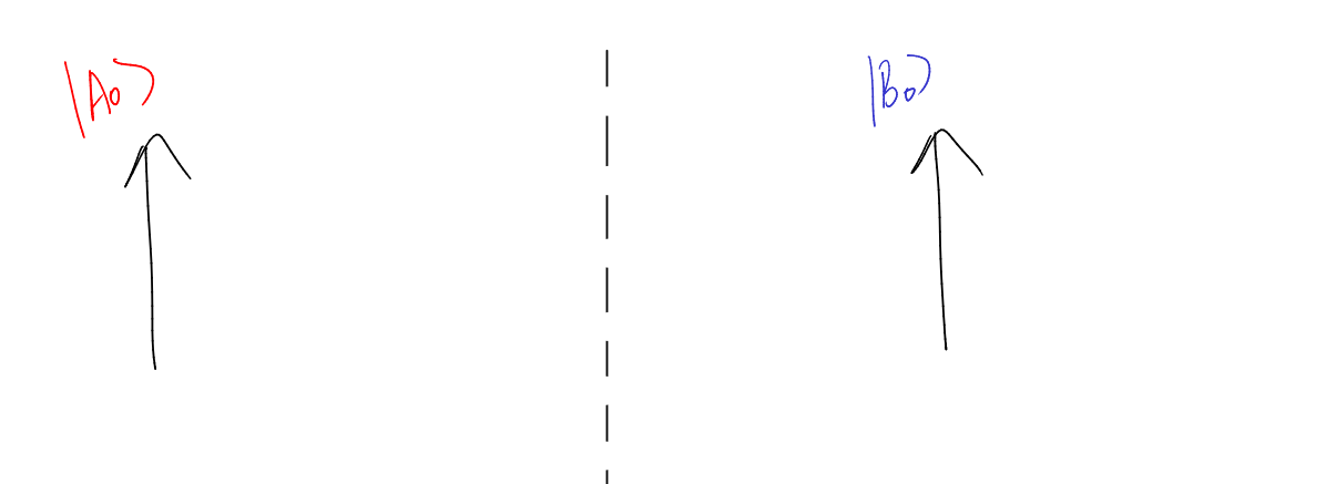
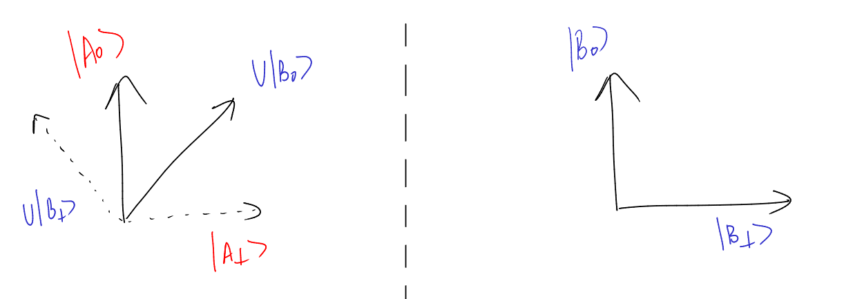
To see this, let us zoom into our Hilbert space. Consider these two diagrams each representing a different portion of the large Hilbert space, and our vectors \(\vert A_0 \rangle\) and \(\vert B_0 \rangle\) lie here.
Now, consider the vector \(U\vert B_0\rangle\) added to the image:
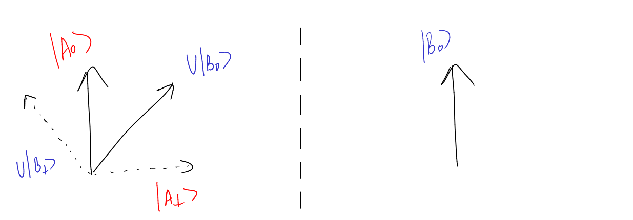 Note that vectors \(\vert A_0\rangle\) and \(U|B_0\rangle\) both define a plane. Thus, we have well-defined vectors \(\vert A_\perp\rangle\) and \(U \vert B \rangle_\perp = U \vert B_\perp \rangle\) that lie on the same plane on the left that we’ve defined (upto scalar multiple). Thus, this fixes the vector \(\vert B_\perp \rangle\) which is the pre-image of the vector \(U \vert B_\perp \rangle\). The vectors \(\vert B_0 \rangle\) and \(\vert B_\perp \rangle\) also define a plane!
Now, while \(U\) acts on a large Hilbert space, we can always ask: what happens when \(U\) acts on a vector in the \(\vert B_0\rangle, \vert B_{\perp} \rangle\) plane? Well, it takes it to the \(\vert A_0 \rangle, \vert A_\perp \rangle\) plane! We can write the matrix \(U\) in these two bases expressing exactly this. Recall that we denoted \(\langle A_0 \vert U \vert B_0 \rangle\) by \(a\). We denote the action of \(U\) in this subspace as \(R(a)\):
\[\begin{array}{ccc} && \begin{array}{cccc} \langle B_0 \vert &&& \langle B_\perp \vert \\ \end{array} \\ R(a) = & \begin{array} & \vert A_0 \rangle \\ \vert A_\perp \rangle \end{array} & \left[ \begin{array}{cc} a & \sqrt{1-a^2} \\ \sqrt{1 - a^2} & -a \end{array} \right] \end{array}\]It turns out that \(R\) can be decomposed as follows:
\[-ie^{i\frac{\pi}{4}Z}W(a)e^{i\frac{\pi}{4}Z}\]which is basically a signal rotation flanked by two \(Z\) rotations, upto a scalar.
So far, we have shown that the \(U\) matrix we are provided with looks like a signal rotation flanked by two \(Z\) rotations, if we worry only about its action in a \(2\)-dimensional input and output subspace. Now, we will show that if we do something similar to the other two operators we have been provided, namely take the matrices \(e^{i\phi \vert A_0 \rangle \langle A_0 \vert}\) and \(e^{i \psi \vert B_0 \rangle \langle B_0 \vert}\) and only worry about what they do in a small subspace, they resemble the signal-processing (or \(Z\) rotation) matrices!
What is the matrix \(e^{i\phi \vert A_0 \rangle \langle A_0 \vert}\)? Let us consider how it would look in some diagonal basis containing \(\vert A_0 \rangle\) and \(\vert A_\perp \rangle\):
\[\begin{array}{ccc} && \begin{array}{ccc} \langle A_0 \vert & \langle A_\perp \vert & \dots\\ \end{array} \\ e^{i\phi \vert A_0 \rangle \langle A_0 \vert} = & \begin{array}{ccc} \vert A_0 \rangle \\ \vert A_\perp \rangle \\ \vdots \end{array} & \left[ \begin{array}{ccc} e^{i\phi} & 0 & \dots \\ 0 & 1 & \\ \vdots & & \ddots \\ \end{array} \right] \end{array}\]Thus, in the \(2\)-dimensional subspace spanned by \(\vert A_0 \rangle\) and \(\vert A_\perp \rangle\), the action of the above operator is \(e^{i\phi} \vert A_0 \rangle \langle A_0 \vert + \vert A_\perp\rangle \langle A_\perp \vert = e^{i\phi} \left(\vert A_0 \rangle \langle A_0 \vert + e^{-i \phi} \vert A_\perp\rangle \langle A_\perp \vert \right)\). Hence, in this basis, it is a rotation about \(\vert A_0 \rangle \langle A_0 \vert\) by an angle \(-\phi\). (This is easy to see if you imagine a Bloch sphere with the \(\vert 0 \rangle \langle 0 \vert\) being \(\vert A_0 \rangle \langle A_0 \vert\), and the \(\vert 1 \rangle \langle 1 \vert\) being \(\vert A_\perp \rangle \langle A_\perp \vert\)). The phase operator for \(\vert B_0 \rangle\) is analogously a rotation in the \(\vert B_0\rangle, \vert B_\perp \rangle\) qubit. You can see where this is going, then. If you interleave the original \(U\) given to you with the phase operators, and only ask what they do to a \(2\)-dimensional subspace, you recover the QSP formalism (some scalar factors have been omitted):
\[\begin{array}{cc} & \begin{array}{cc} \langle A_0 \vert & \langle A_\perp \vert \\ \end{array} \\ \begin{array} & \vert A_0 \rangle \\ \vert A_\perp \rangle \end{array} & \left[ \begin{array}{cc} 1 & 0 \\ 0 & e^{-i\psi} \end{array} \right] \end{array} \begin{array}{cc} & \begin{array}{cccc} \langle B_0 \vert &&& \langle B_\perp \vert \\ \end{array} \\ \begin{array} & \vert A_0 \rangle \\ \vert A_\perp \rangle \end{array} & \left[ \begin{array}{cc} a & \sqrt{1-a^2} \\ \sqrt{1 - a^2} & -a \end{array} \right] \end{array} \begin{array}{cc} & \begin{array}{cc} \langle B_0 \vert & \langle B_\perp \vert \\ \end{array} \\ \begin{array} & \vert B_0 \rangle \\ \vert B_\perp \rangle \end{array} & \left[ \begin{array}{cc} 1 & 0 \\ 0 & e^{-i\psi} \end{array} \right] \end{array}\]Above, we’ve applied a phase rotation, the unitary and another phase rotation (pay attention to the labels of the matrices), and asked how this looks like when I look at the input space \(span\{\vert B_0\rangle, \vert B_\perp \rangle\}\) and output space \(span\{\vert A_0\rangle, \vert A_\perp\rangle \}\). And it looks exactly like the QSP interleaving of a signal operator with its signal processing operators! More precisely, the rightmost matrix above is \(R_z(-\psi)\), the middle matrix is \(-ie^{i\frac{\pi}{4}Z}W(a)e^{i\frac{\pi}{4}Z}\), (the \(Z\) rotations that flank the signal can be combined with the signal-processing operators), and the rightmost matrix is once again \(R_z(-\phi)\). Thus, upon building a circuit \(Q\) by interleaving these as discussed in the signal processing section, one can pick phases such that \(\langle A_0 \vert Q \vert B_0\rangle = P(a)\), where \(P(a)\) is any polynomial that fits the QSP polynomial constraints.
Grover’s search from the generalised QSP
Now is time for some real magic 3.
Let’s recall the quantum search problem, and Grover’s algorithm to solve the problem. One formulation of the search problem is that you are provided with an oracle that gives a \('-'\) sign to a particular state only and acts as the identity on other states. Let’s call this state \(\vert A_0 \rangle\). Thus, this oracle can be written as \(e^{i\pi \vert A_0 \rangle \langle A_0 \vert}\).
Grover’s algorithm then involves applying \(H\) on the starting state \(\vert 0 \rangle\), and then alternatingly applying the Grover’s oracle, and the inversion about mean.
What is the inversion about mean? It is the operator \(I - 2 \vert \psi \rangle \langle \psi \vert\), where \(\vert \psi \rangle\) is the completely superposed state. However, this can be written as:
\[I - 2 \vert \psi \rangle \langle \psi \vert = H (I - 2 \vert 0 \rangle \langle 0 \vert) H = H (e^{i\pi \vert 0 \rangle \langle 0 \vert}) H\]where \(H\) is the Hadamard gate on all qubits. Awesome! How does the sequence of gates used in Grover’s search look like?
\[... H (e^{i\pi \vert 0 \rangle \langle 0 \vert}) H (e^{i\pi \vert A_0 \rangle \langle A_0 \vert}) H\]Is this starting to look familiar? Let us write the above sequence in signal processing terms.
\[... U (e^{i\psi \vert B_0 \rangle \langle B_0 \vert}) U (e^{i\phi \vert A_0 \rangle \langle A_0 \vert}) U\]Ta da! That’s it! So, the \(H\) we apply in Grover’s search is essentially the signal \(U\). The Grover’s oracle is the signal processing operator \(e^{i \phi \vert A_0 \rangle \langle A_0 \vert}\), except you’re only allowed a phase of \(\pi\). The other signal processing operator \(e^{i \phi \vert 0 \rangle \langle 0 \vert}\) is essentially the \(\vert B_0 \rangle\) operator with \(\vert B_0 \rangle = \vert 0 \rangle\).
The elements of the QSP that are given to us as input, and the elements that we actually have control over are probably different from what one would expect from a signal processing problem. Here, we are free to choose the “signal”, which we chose as the Hadamard, and we’re free to choose one of the signal processing operators (the rotation about \(\vert B_0 \rangle\)). However, the other signal processing operator (rotation about \(\vert A_0 \rangle\)) is the Grover oracle that is given to us.
So, we still need to answer: why do we choose our signal operator as the Hadamard, and how does this relate to the polynomial-designing portion of QSP? Assume that we did choose Hadamard. Then what is the value of \(a = \langle A_0 \vert H \vert 0 \rangle\)? Remember, we don’t know what \(\vert A_0 \rangle\) is. However, note that we do know that it is a computational basis state. And because we used the Hadamard, this is good for us, and we immediately have \(a = \frac{1}{\sqrt{N}}\), where \(N = 2^n\) and \(n\) is the number of qubits, irrespective of what \(\vert A_0\rangle\) is !
Now, what is our aim? We want to start at the \(\vert 0\rangle\) state, and construct some circuit \(Q\) such that, the state at the end is \(\vert A_0 \rangle\). In other words, we require \(\langle A_0 \vert Q \vert 0 \rangle = 1\). We know that for the particular \(U\) that we picked, which is \(H\), we have \(a = \frac{1}{\sqrt{N}}\). Thus, we need to find phases such that \(P(1/\sqrt N) = 1\), where the polynomial \(P(a) = \langle A_0 \vert Q(a) \vert 0 \rangle\).
It turns out, a polynomial that satisfies this is an \(O(\sqrt N)\)-degree polynomial that can be constructed by having \(\pi\) rotations for all the signal-processing operators. This is a good thing, because every alternate signal-processing operator was fixed at \(\pi\) to begin with. Aand that is how Grover’s original algorithm is obtained as an instance of signal-processing.
Casting Grover’s as a QSP problem leads to pretty cool insights. One of them is that: “there may be other polynomials that satisfy our bare requirement, which is \(P(1/\sqrt N) = 1\), but behave better than Grover’s”. In particular, perhaps, repeating the building blocks too many times would not move the state vector too far from the true solution: which is not true for Grover’s original algorithm and has catastrophic effects. Such thinking led to the fixed point version of the Grover’s algorithm.
It is tempting to ask–can one find a lower degree QSP polynomial which also satisfies the \(P(1/\sqrt N)\) constraint? Since the degree of the polynomial directly relates to the number of times the oracle is called, one would then get a more efficient solution to quantum search! However, this tantalizing possibility is ruled out by lower bounds on the search problem: a lower degree QSP polynomial that satifies our condition simply does not exist!
And this depressing thought which saddened me for a few weeks is a good place to end this article.
-
There are two more constraints on \(P(a)\). One of them is that its parity must be \(d \% 2\). The second constraint is with relation to another polynomial, which is part of the \(\langle 0 \vert Q \vert 1 \rangle\) entry of the matrix, and is explained formally in the Grand Unification paper. ↩
-
I’m still unsure why this promise is important. One thing I note is that when \(a\) is \(0\), this reduces the rotation matrix \(R(a)\) (defined a few paragraphs below) to an \(X\) rotation, and intuitively, this may not allow one to have \(\langle A_0 \vert Q \vert B_0 \rangle\) to be any QSP polynomial. ↩
-
The term “magic”, also has a technical definition in quantum computing, that we are not referring to here. I’ll say this though: the people coming up with these names (see teleportation) are at least in part responsible for the hype the field sees! ↩