The Hadamard Sandwich
The Hadamard Sandwich is a neat quantum circuit trick that shows up in several quantum algorithms! In this post, we will cover what the Hadamard Sandwich is, and its application in (1) the swap test, (2) the fixed point quantum search algorithm, and (3) the eigenvalue threshold algorithm.
What is the Hadamard Sandwich?
Let us first define a type of quantum gate that is our main focus in this post.
The projector controlled-unitary gate: Let \(U\) be a \(2^n \times 2^n\) unitary matrix (in other words, a quantum gate on \(n\) qubits), and let \(P\) be a \(2^m \times 2^m\) orthogonal projector. Then \(P\)-controlled \(U\) is the following \(m+n\) qubit gate (which you can check is unitary):
\[P \otimes U + (I-P) \otimes I.\]The CNOT gate is an example of a projector-controlled unitary gate, where the projector is \(\mid 1 \rangle \langle 1 \mid\) and the unitary is \(X\):
\[| 1 \rangle \langle 1| \otimes X + | 0 \rangle \langle 0 | \otimes I.\]When the projector \(P\) is just \(\mid 1\rangle \langle 1 \mid\)—as in the above case—we simply call it a controlled-\(U\) gate.
Assume you have access to the gate on the left, that is, a controlled-\(U\) acting on \(n+1\) qubits, where you are promised that \(U\) has only eigenvalues \(+1\) and \(-1\). Let \(\{\mid e_i \rangle\}_i\) be an orthogonal basis for the eigenspace of \(U\) with eigenvalue \(-1\), and let \(P = \sum_i \mid e_i \rangle \langle e_i \mid\). That is, \(P\) is a projector into the \(-1\) eigenspace of \(U\).
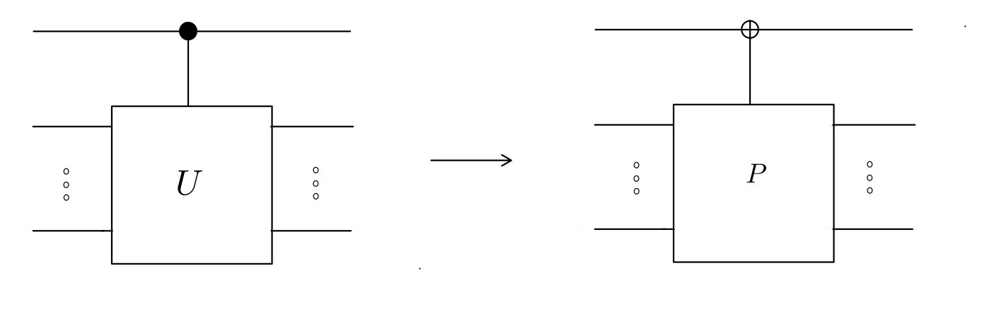
Then, the Hadamard Sandwich (no, I haven’t seen this term used anywhere), is a trick to convert the gate on the left (a controlled-\(U\)),
\[| 1 \rangle \langle 1| \otimes U + | 0 \rangle \langle 0 | \otimes I.\]to the gate on the right (a \(P\)-controlled \(X\)),
\[X \otimes P + I \otimes (I-P).\]Crucially, notice that on the left, \(U\) is controlled by the top qubit, and acts on all the bottom qubits. However, for the gate on the right, the \(X\) gate is controlled by all the bottom qubits but acts on the top qubit.
How is this accomplished? By simply sandwiching the top qubit of the gate on the left with Hadamards!
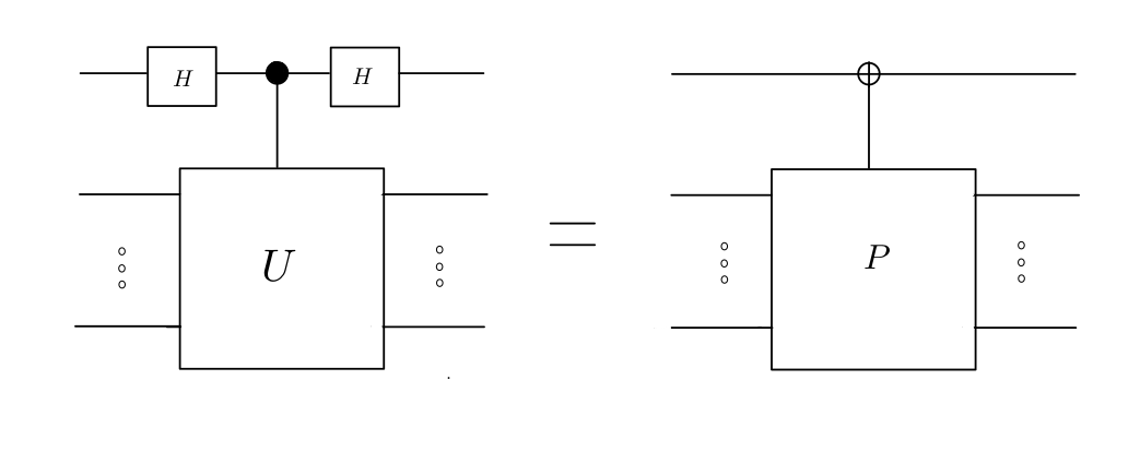
To prove this, let us write \(U\) in terms of its \(+1\) and \(-1\) eigenvectors:
\[U = \sum_j |a_j \rangle \langle a_j | - \sum_i |e_i \rangle \langle e_i | = (I-P) - P = I - 2P\]Applying the Hadamard Sandwich to gate on the left, we have,
\[H| 1 \rangle \langle 1|H \otimes U + H| 0 \rangle \langle 0 |H \otimes I.\] \[= \frac 1 2 (|0\rangle \langle 0| + |1\rangle \langle 1| - |0 \rangle \langle 1| - |1 \rangle \langle 0 |)\otimes U + \frac 1 2(|0\rangle \langle 0| + |1\rangle \langle 1| + |0 \rangle \langle 1| + |1 \rangle \langle 0 |) \otimes I.\] \[= (|0 \rangle \langle 1| + |1 \rangle \langle 0 |)\otimes \Big(\frac{I-U}2 \Big) + (|0\rangle \langle 0| + |1\rangle \langle 1|) \otimes \Big(\frac{I+U}2\Big)\] \[= X \otimes P + I \otimes (I-P)\]Thus, the original controlled-\(U\) has been converted to a \(P\)-controlled-\(X\). Now let’s look at where this idea shows up!
The Swap Test
The Swap Test is a circuit that can be used to compute the (absolute value of) inner product of two vectors given as quantum states. To accomplish this, both states and an ancilla qubit in \(\mid 0\rangle\) state are given as input to a Hadamard-sandwiched controlled-SWAP:
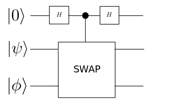
After applying the circuit, the probability of measuring the ancilla as \(\mid 1 \rangle\) is then \(\frac{1 - \Vert \langle \psi \mid \phi \rangle \Vert ^2}2\), from which the absolute value of the inner product can be obtained.
We first prove this directly. The initial state is
\[|0\rangle |\psi \rangle |\phi \rangle\]Upon applying Hadamard,
\[\frac 1 {\sqrt 2} \big(|0\rangle + |1\rangle \big) |\psi \rangle |\phi \rangle\]After the controlled swap,
\[\frac 1 {\sqrt 2} \big(|0\rangle |\psi \rangle |\phi \rangle + |1\rangle |\phi \rangle |\psi \rangle \big)\]Hadamard again,
\[| \alpha \rangle = \frac 1 2 \bigg(|0\rangle \big(|\psi \rangle |\phi \rangle + |\phi \rangle |\psi \rangle \big) + |1\rangle \big(|\psi \rangle |\phi \rangle - |\phi \rangle |\psi \rangle \big) \bigg)\]The probability of measuring the ancilla as \(\mid 1 \rangle\) is
\[\langle \alpha | \big(|1\rangle \langle 1| \otimes I \big) |\alpha \rangle\] \[= \frac 1 4 \big(\langle \psi | \langle \phi | - \langle \phi | \langle \psi | \big) \big(|\psi \rangle |\phi \rangle - |\phi \rangle |\psi \rangle \big)\] \[= \frac {1 - \Vert \langle \psi \vert \phi \rangle \Vert^2} 2\]We can also analyse the swap test through the lens of the Hadamard Sandwich. We do it here for the case where \(\vert \psi\rangle\) and \(\vert \phi\rangle\) are both \(1\)-qubit states. An eigenbasis for the \(2\)-qubit SWAP gate is the Bell basis, where the state \(\vert \beta \rangle = \frac 1 {\sqrt 2} \big (\vert 01 \rangle - \vert 10 \rangle \big )\) has an eigenvalue \(-1\) and the rest have eigenvalues \(+1\).
Now, we know that the Hadamard Sandwich has converted the controlled SWAP into a projector-controlled \(X\) gate. And since \(\vert \beta \rangle\) is the only eigenvector with \(-1\) eigenvalue, the projector is essentially \(\vert \beta \rangle \langle \beta \vert\).
We rewrite the circuit as a projector-controlled \(X\) gate, and thus, we need to compute the probability of measuring the ancilla as \(\vert 1 \rangle\) in the following state:
\[\Big (X \otimes |\beta \rangle \langle \beta | + I \otimes (I- |\beta \rangle \langle \beta |) \Big )|0 \rangle | \psi \phi \rangle\]which is
\[\Bigg \Vert \Big ( |1\rangle \langle 1 | \otimes I \Big )\Big (X \otimes |\beta \rangle \langle \beta | + I \otimes (I- |\beta \rangle \langle \beta |) \Big )|0 \rangle | \psi \phi \rangle \Bigg \Vert^2\] \[= \Bigg \Vert \Big ( |1\rangle \langle 1 | \otimes I \Big ) \Big (|1\rangle \otimes |\beta \rangle \langle \beta | \psi \phi \rangle \Big ) \Bigg \Vert^2\] \[= \Bigg \Vert |1\rangle \otimes |\beta \rangle \langle \beta | \psi \phi \rangle \Bigg \Vert^2\] \[= \frac 1 2\langle \psi \phi \vert \big ( |01 \rangle - |10 \rangle\big) \big( \langle 01 | - \langle 10 | \big) | \psi \phi \rangle\] \[\frac 1 2 \big(\psi_0^* \phi_1^* - \psi_1^*\phi_0^*) \big(\psi_0 \phi_1 - \psi_1\phi_0)\] \[= \frac 1 2 \big( \psi_0^*\phi_1^*\psi_0\phi_1 + \psi_1^*\phi_0^*\psi_1\phi_0 - \psi_0^*\phi_1^*\psi_1\phi_0 - \psi_1^*\phi_0^*\psi_0\phi_1 \big ), \tag{1}\]where \(\psi_0 \equiv \langle 0 \vert \psi \rangle\), and so forth. However, notice that we have \(\langle \psi \vert \psi \rangle \langle \phi \vert \phi \rangle = 1\)
Thus,
\[( \psi_0^*\psi_0 + \psi_1^* \psi_1 ) (\phi_0^* \phi_0 + \phi_1^* \phi_1) = 1\] \[\psi_0^*\psi_0\phi_0^*\phi_0 + \psi_0^*\psi_0\phi_1^*\phi_1 + \psi_1^*\psi_1\phi_0^*\phi_0 + \psi_1^* \psi_1 \phi_1^*\phi_1 = 1\]and
\[\psi_0^*\psi_0\phi_1^*\phi_1 + \psi_1^*\psi_1\phi_0^*\phi_0 = 1 - \psi_0^*\psi_0\phi_0^*\phi_0 - \psi_1^* \psi_1 \phi_1^*\phi_1 \tag{2}\]Thus, substituting Eq\((2)\) in \((1)\), we have
\[= \frac 1 2 \bigg( 1 - \big ( \psi_0^*\psi_0\phi_0^*\phi_0 + \psi_1^* \psi_1 \phi_1^*\phi_1 + \psi_0^*\phi_1^*\psi_1\phi_0 + \psi_1^*\phi_0^*\psi_0\phi_1 \big ) \bigg )\] \[= \frac 1 2 \bigg( 1 - \big ( \psi_0\phi_0^* + \psi_1\phi_1^* \big ) \big ( \psi_0^*\phi_0 + \psi_1^*\phi_1 ) \bigg )\] \[= \frac {1 - \Vert \langle \psi \vert \phi \rangle \Vert^2} 2\]which is the original expression obtained in the first method! Thus, another way of thinking about the swap test is that the ancilla qubit is flipped based on how big a component of \(\vert \psi \phi \rangle\) lies along the state \(\vert \beta \rangle\): the bigger this component, the smaller the inner product between \(\vert \psi \rangle\) and \(\vert \phi \rangle\) and vice versa. I would like to understand this connection better.
The Fixed-Point Grover’s Search
The next application where the Hadamard Sandwich shows up is in improving the Grover’s search algorithm. The Grover’s search suffers from the “overcooking problem”, that is, too many applications of the Grover iterate (the building block of the algorithm) can cause the final solution to start getting worse rather than better. A fixed-point optimal version of the algorithm was discovered in 2014 by Yoder et al., which does not suffer from the same issue. We won’t discuss the details of the algorithm here, which are also explained well in Martyn et al., but mention one subroutine that occurs in the algorithm.
In the quantum search problem, we assume the existence of a unitary that flips the target states, but acts as identity on all other states. That is, for all basis states \(\vert \alpha \rangle\), we have
\(U_G \vert \alpha\rangle = - \vert \alpha\rangle\) if \(\vert \alpha\rangle\) is a target, and
\(U_G \vert \alpha\rangle = \vert \alpha\rangle\) otherwise.
In the fixed point version, we require a unitary that gives a phase of our choice, rather than \(-1\), to the target states. Given a controlled version of \(U_G\), we wish to apply \(U_G'\) such that
\(U_G' \vert \alpha\rangle = e^{i\theta} \vert \alpha\rangle\) if \(\vert \alpha\rangle\) is a target, and
\(U_G' \vert \alpha\rangle = \vert \alpha\rangle\) otherwise.
Given that the unitary \(U_G\) has only eigenvalues \(-1\) and \(+1\), this already smells like a Hadamard Sandwich, and indeed, this transformation is accomplished by using the Hadamard Sandwich twice:
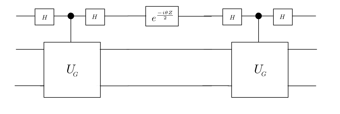
This circuit has three parts. First, we apply a Hadamard-Sandwiched controlled-\(U_G\). Then, we apply a \(Z\) rotation on the first qubit, followed by another Hadamard-Sandwiched controlled-\(U_G\).
Assume \(\vert 0\rangle\) is input as the top qubit. The idea is that the first Hadamard Sandwich flips the top qubit to \(\vert 1\rangle\) only if the other qubits are in the \(-1\) eigenspace of \(U_G\). The rotation gate, which is \(e^{\frac{-i\theta}{2}}\vert 0 \rangle \langle 0 \vert + e^{\frac{i\theta}{2}}\vert 1 \rangle \langle 1 \vert = e^{\frac{-i\theta}{2}}\big(\vert 0 \rangle \langle 0 \vert + e^{i \theta}\vert 1 \rangle \langle 1 \vert\big)\) is then applied, which gives a phase to \(\vert 1 \rangle\). The final Hadamard Sandwich essentially makes the top qubit \(\vert 0 \rangle\) again, attaching the phase to the \(-1\)-eigenspace, producing \(U_G'\). To prove this, (1) we first write the circuit expression as is, (2) then take global phase common, and (3) replace the Hadamard Sandwich controlled-\(U_G\) with a projector-controlled-\(X\):
\[\big(H|0\rangle \langle 0|H \otimes I + H|1\rangle \langle 1|H \otimes U_G \big) \bigg(\big(e^{\frac{-i\theta}{2}}\vert 0 \rangle \langle 0 \vert + e^{\frac{i\theta}{2}}\vert 1 \rangle \langle 1 \vert \big) \otimes I \bigg) \big(H|0\rangle \langle 0|H \otimes I + H|1\rangle \langle 1|H \otimes U_G \big)\] \[= e^{-\frac{i\theta}{2}} \big(H|0\rangle \langle 0|H \otimes I + H|1\rangle \langle 1|H \otimes U_G \big) \bigg(\big(\vert 0 \rangle \langle 0 \vert + e^{i \theta}\vert 1 \rangle \langle 1 \vert \big) \otimes I \bigg)\big(H|0\rangle \langle 0|H \otimes I + H|1\rangle \langle 1|H \otimes U_G \big)\] \[= e^{-\frac{i\theta}{2}} \big( X \otimes P + I \otimes (I-P)\big) \bigg(\big(\vert 0 \rangle \langle 0 \vert + e^{i \theta}\vert 1 \rangle \langle 1 \vert \big) \otimes I \bigg)\big(X \otimes P + I \otimes (I-P)\big)\] \[= e^{-\frac{i\theta}{2}} \big( X \otimes P + I \otimes (I-P)\big) \bigg(\big(\vert 0 \rangle \langle 1 \vert + e^{i \theta}\vert 1 \rangle \langle 0 \vert \big) \otimes P + \big(\vert 0 \rangle \langle 0 \vert + e^{i \theta}\vert 1 \rangle \langle 1 \vert \big) \otimes (I-P) \bigg)\] \[= e^{-\frac{i\theta}{2}}\bigg(\big(\vert 1 \rangle \langle 1 \vert + e^{i \theta}\vert 0 \rangle \langle 0 \vert \big) \otimes P + \big(\vert 0 \rangle \langle 0 \vert + e^{i \theta}\vert 1 \rangle \langle 1 \vert \big) \otimes (I-P) \bigg)\] \[= e^{-\frac{i\theta}{2}} \bigg(|0\rangle \langle 0| \otimes \big(e^{i \theta} P + (I-P)\big ) + |1\rangle \langle 1| \otimes \big(P + e^{i \theta} (I-P)\big ) \bigg)\] \[= e^{-\frac{i\theta}{2}} \bigg(|0\rangle \langle 0| \otimes U_G' + |1\rangle \langle 1| \otimes \big(P + e^{i \theta} (I-P)\big ) \bigg)\]Thus, upto global phase, the circuit applies \(U_G'\) when the top qubit is set to \(\vert 0\rangle\).
The Eigenvalue Threshold Problem
The statement of this problem is: given a Hamiltonian \(\mathcal{H}\), and a threshold value \(\lambda_{th}\), return whether or not the Hamiltonian has any eigenvalues less than \(\lambda_{th}\). To solve this problem, we are also given access to a vector which has significant overlap with the low eigenvalues of \(\mathcal{H}\), should they exist. That is, we have access to \(| \psi \rangle\) such that \(\Vert \pi |\psi \rangle \Vert \geq c\), where \(\pi = \sum_i \vert l_i \rangle \langle l_i \vert\), and \(\vert l_i \rangle\) are eigenvectors of \(\mathcal{H}\) that have eigenvalues less than \(\lambda_{th}\).
Once again, without getting into the details which are explained in Martyn et al., we simply state that applying the QSVT method to this problem leaves us with a final controlled-\(U\) that has the same eigenvectors as \(\mathcal{H}\), but with its eigenvalues tweaked: an eigenvalue is now close to \(-1\) if the original eigenvalue was less than \(\lambda_{th}\), and is close to \(1\) if the original eigenvalue was larger than \(\lambda_{th}\).
Thus, to decide the eigenvalue threshold problem, we are left to (roughly) differentiate between a controlled version of the identity matrix, and a controlled version of a unitary with \(-1\)’s and \(1\)’s on its diagonal.
Here, the Hadamard Sandwich is once again used to convert the controlled-\(U\) to a \(\pi\)-controlled \(X\)—and when \(\vert \psi \rangle\) is given as input to this circuit,
- If none of the eigenvalues of \(\mathcal{H}\) were greater than \(\lambda_{th}\), then after QSVT, the unitary does not have any \(-1\) eigenvalues, \(\pi\) is a null projector, and the top qubit is not flipped.
- If at least one of the eigenvalues of \(\mathcal{H}\) was less than \(\lambda_{th}\), then after QSVT, the unitary has some \(-1\) eigenvalues, \(\pi\) is a projector into this \(-1\)-eigenspace, with some probability, the top qubit is flipped.
Thus, measuring the top qubit can be used to differentiate between the two cases.
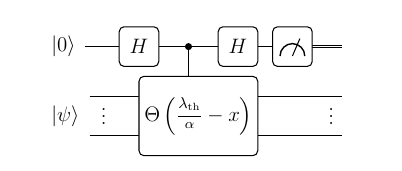
The above image depicting the Hadamard Sandwich being used in the Eigenvalue Threshold problem is taken from the Martyn et al. paper.
Conclusion
In this post, we saw how the simple primitive of converting a controlled-\(U\) to a \(P\)-controlled-\(X\) appears in quantum computing in accomplishing several different tasks. This primitive also appears as part of the QSVT-based phase estimation algorithm. Let me know in the comments if you spot this being used in any other algorithm in quantum computing!